Extracción y redifusión de la EPA

Lluís Revilla

Recursos

Taller Congreso R

• Conectar R and DataWrapper

• Com utilitzar R per treballar amb microdades

Otros:

• Scripts

• Esta web

¿ Datos ?

Website:

https://www.ine.es/jaxiT3/dlgExport.htm?t=4248&L=0

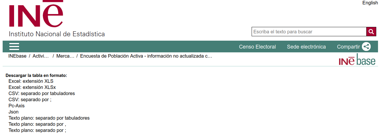
Descargar datos

• XLS: https://www.ine.es/jaxiT3/files/t/es/xls/4248.xls
• XLSX: https://www.ine.es/jaxiT3/files/t/es/xlsx/4248.xlsx
• TSV (\t): https://www.ine.es/jaxiT3/files/t/es/csv_bd/4248.csv
• CSV (;): https://www.ine.es/jaxiT3/files/t/es/csv_bdsc/4248.csv
• Pc-Axis: https://www.ine.es/jaxiT3/files/t/es/px/4248.px
• JSON: https://servicios.ine.es/wstempus/jsCache/es/DATOS_TABLA/4248?tip=AM&
• TSV (\t): https://www.ine.es/jaxiT3/files/t/es/csv/4248.csv
• CSV (,): https://www.ine.es/jaxiT3/files/t/es/csv_c/4248.csv
• CSV (;): https://www.ine.es/jaxiT3/files/t/es/csv_sc/4248.csv

En R

url <- "https://www.ine.es/jaxiT3/files/t/es/csv_bdsc/4248.csv"
download.file(url, file.path("data", basename(url)))

Descargar varios archivos

download_file <- function(id) {
  read.csv(paste0("https://www.ine.es/jaxiT3/files/t/es/csv_bdsc/",id, ".xls"), 
           sep = ";", header = 1,
                  dec = ",", check.names = FALSE)
}
df <- download_file(4248)
# df <- download_file(181)

Descargar ~1000 archivos:

files <- sapply(1:1000, function(x){
  # url <- paste0("https://www.ine.es/jaxiT3/dlgExport.htm?t=", x, "&L=0")
  url <- paste0("https://www.ine.es/jaxiT3/files/t/es/csv_bdsc/", x, ".xls?nocab=1")
  file_path <- paste0("data/", x, ".csv")
  download.file(url, destfile = file_path)
  if (file.exists(file_path)) {
    file_path
  } else {
    NULL
  }
})

EPA

EPA website:

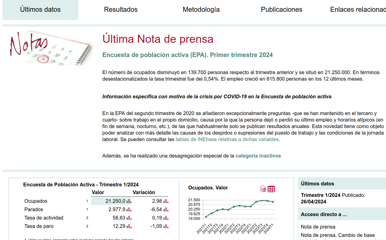
EPA screenshot

Descargar EPA

Where is the data?

EPA microdatos screenshot

EPA desde R

download_epa <- function(trimester, year) {
  
  stopifnot(nchar(year) == 2)
  stopifnot(nchar(trimester) == 1L)
  url <- paste0("https://www.ine.es/ftp/microdatos/epa/datos_", 
               trimester, "t", year, ".zip")
  file_zip <- file.path("data", basename(url))
  download.file(url, file_zip)
  file_zip
}
EPA_4t23 <- download_epa("4", "23")

Cargar los datos

unzip(EPA_4t23, exdir = "data/EPA_4t23/")
obj <- load("data/EPA_4t23/R/EPA_2023T4.RData")
obj

[1] "Microdatos" "Metadatos" 

# View(Metadatos)
micro <- as.data.frame(Microdatos)
micro[1:5, 1:5]

  CICLO CCAA PROV NVIVI NIVEL
1   205   16   01 00001     1
2   205   16   01 00002     1
3   205   16   01 00003     1
4   205   16   01 00003     1
5   205   16   01 00003     2

¿Qué hay?

library("MicroDatosEs")
variables <- read.delim2(system.file("metadata", "epa_mdat2.txt", 
                        package = "MicroDatosEs"))
columnas <- read.delim2(system.file("metadata", "epa_mdat1.txt", 
                        package = "MicroDatosEs"))
head(variables)

    var tipo nulo llave                    valor
1 CICLO    N   NA  <NA>                         
2  CCAA    D   NA     1                Andalucía
3  CCAA    D   NA     2                   Aragón
4  CCAA    D   NA     3 Asturias (Principado de)
5  CCAA    D   NA     4         Baleares (Islas)
6  CCAA    D   NA     5                 Canarias

head(columnas)

    var start end width                                                   descr
1 CICLO     1   3     3                                   Período de referencia
2  CCAA     4   5     2                                      Comunidad autónoma
3  PROV     6   7     2                                               Provincia
4 NVIVI     8  12     5                          Número de orden de la vivienda
5 NIVEL    13  13     1 Variable que indica el nivel del registro en el fichero
6 NPERS    14  15     2                                    Número de la persona

Los datos

library("dplyr")
our_data <- micro |> 
  count(CCAA, PROV) |> 
  group_by(CCAA) |> 
  mutate(n_provincias = n_distinct(PROV)) |> 
  ungroup()

head(our_data)

# A tibble: 6 × 4
  CCAA  PROV      n n_provincias
  <chr> <chr> <int>        <int>
1 01    04     1829            8
2 01    11     2422            8
3 01    14     1516            8
4 01    18     2018            8
5 01    21     1218            8
6 01    23     1720            8

CCAA

ccaa <- variables |> filter(var  == "CCAA") |> 
  tidyr::pivot_wider(names_from = var, values_from = valor) |> 
  mutate(llave = if_else(nchar(llave) == 1L, paste0("0", llave), llave)) |> 
  rename(ca = CCAA) |> 
  mutate(ca = trimws(ca)) |> 
  select(-tipo, -nulo)
head(ccaa)

# A tibble: 6 × 2
  llave ca                      
  <chr> <chr>                   
1 01    Andalucía               
2 02    Aragón                  
3 03    Asturias (Principado de)
4 04    Baleares (Islas)        
5 05    Canarias                
6 06    Cantabria               

Provincias

prov <- variables |> filter(var  == "PROV") |> 
  tidyr::pivot_wider(names_from = var, values_from = valor) |> 
  mutate(llave = if_else(nchar(llave) == 1L, paste0("0", llave), llave)) |> 
  rename(provincia = PROV) |> 
  mutate(provincia = trimws(provincia)) |> 
  select(-tipo, -nulo)
head(prov)

# A tibble: 6 × 2
  llave provincia
  <chr> <chr>    
1 01    Álava    
2 02    Albacete 
3 03    Alicante 
4 04    Almería  
5 05    Ávila    
6 06    Badajoz  

Juntando

m_ccaa <- merge(our_data, ccaa, 
                by.x = "CCAA", by.y = "llave", 
                sort = FALSE)
m_ccaa_prov <- merge(m_ccaa, prov, 
                     by.x = "PROV", by.y = "llave", 
                     sort = FALSE)
head(m_ccaa_prov)

  PROV CCAA    n n_provincias        ca provincia
1   04   01 1829            8 Andalucía   Almería
2   11   01 2422            8 Andalucía     Cádiz
3   14   01 1516            8 Andalucía   Córdoba
4   18   01 2018            8 Andalucía   Granada
5   21   01 1218            8 Andalucía    Huelva
6   23   01 1720            8 Andalucía      Jaén

Cargar a Google

library("googlesheets4")
gs4_user()
gs <- googlesheets4::gs4_create(name = "EPA", 
                          sheets = m_ccaa_prov,
                          timeZone = "Europe/Madrid")
gs

Data Wrapper

Registrarse en DataWrapper.

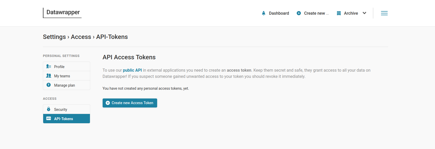
Screenshot for API Access

Cargar de R a DataWrapper

library("DatawRappr")
datawrapper_auth(api_key = Sys.getenv("DATAWRAPPER"))
placeholder <- dw_test_key()
dcc <- dw_create_chart(title = "EPA", type = "tables")
dw_data_to_chart(m_ccaa_prov, dcc$id)

Conectar Google a DataWrapper

epa_gs <- gs4_find("EPA")
url <- paste0("https://docs.google.com/spreadsheets/d/", epa_gs$id[1])

En teoria también por:

library("googledrive")
drive_publish(epa_gs$id[3])

Usa la web

Si no funciona usa el navegador

Ejercicio

¿Te acuerdas de df?

head(df)

  Comunidades y Ciudades Autónomas  Edad        Sexo Periodo Total
1                   Total Nacional Total Ambos sexos  2023T4 11.76
2                   Total Nacional Total Ambos sexos  2023T3 11.84
3                   Total Nacional Total Ambos sexos  2023T2 11.60
4                   Total Nacional Total Ambos sexos  2023T1 13.26
5                   Total Nacional Total Ambos sexos  2022T4 12.87
6                   Total Nacional Total Ambos sexos  2022T3 12.67

Repite el proceso con estos datos.

Repaso

• Descargar datos del INE

• Procesarlos con R

• Subirlos a Google Drive

• Conectarlo con Data Wrapper

Otros

¿Acceso fácil y programable?

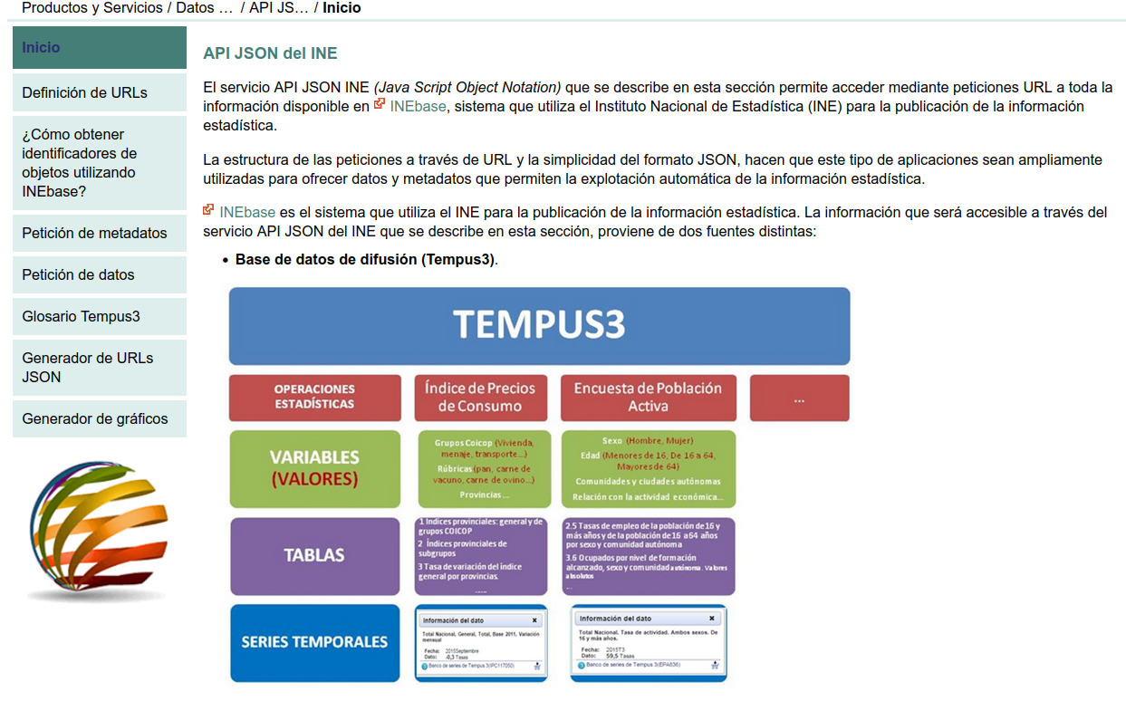
Operaciones disponibles

ine <- download.file("https://servicios.ine.es/wstempus/js/ES/OPERACIONES_DISPONIBLES",
              destfile = "data/operaciones.json")
operaciones <- jsonlite::fromJSON("data/operaciones.json", flatten = TRUE)
head(operaciones)

  Id Cod_IOE                                                 Nombre Codigo  Url
1  4   30147           Estadística de Efectos de Comercio Impagados     EI <NA>
2  6   30211                     Índice de Coste Laboral Armonizado   ICLA <NA>
3  7   30168 Estadística de Transmisión de Derechos de la Propiedad   ETDP <NA>
4 10   30256                                    Indicadores Urbanos     UA <NA>
5 13   30219                Estadística del Procedimiento Concursal    EPC <NA>
6 14   30182                Índices de Precios del Sector Servicios    IPS <NA>

Publicaciones

publicaciones_url <- "https://servicios.ine.es/wstempus/js/ES/PUBLICACIONES"
download.file(publicaciones_url, "data/publicaciones.json")
public <- jsonlite::fromJSON("data/publicaciones.json", flatten = TRUE)
publications <- list2DF(public)
head(publications)

  Id                                                          Nombre
1  1                     Coyuntura Turística Hotelera (EOH/IPH/IRSH)
2  2 Encuesta de ocupación en alojamientos turísticos extrahoteleros
3  3                                               Hipotecas Mensual
4  4                   Indicadores de actividad del sector servicios
5  5                                Índices de Comercio al por menor
6  6                    Índice de Cifras de Negocios en la Industria
  FK_Periodicidad FK_PubFechaAct  Url
1               1          10467 <NA>
2               1          10833 <NA>
3               1          10483 <NA>
4               1          10425 <NA>
5               1          10517 <NA>
6               1          10410 <NA>

Otras publicaciones

download.file("https://servicios.ine.es/wstempus/js/ES/PUBLICACIONFECHA_PUBLICACION/6?det=15",
              destfile = "data/fechapub6.json")
fechas <- jsonlite::fromJSON("data/fechapub6.json", flatten = TRUE)
download.file("https://servicios.ine.es/wstempus/js/ES/PUBLICACIONFECHA_PUBLICACION/7?det=2",
              destfile = "data/fechapub7.json")
fechas7 <- jsonlite::fromJSON("data/fechapub7.json", flatten = TRUE)
download.file("https://servicios.ine.es/wstempus/js/ES/PUBLICACIONFECHA_PUBLICACION/8?det=2",
              destfile = "data/fechapub8.json")
fechas8 <- jsonlite::fromJSON("data/fechapub8.json", flatten = TRUE)